Explain the lumen method for general lighting
When a room is illuminated by many lamps and fittings another method would lead to a very lengthy and cumbersome calculation.
If the fittings are positioned in a regular array, an entirely different, much simpler method can be followed, based on the concept of utilization factor (UF).
This is simply the ratio of the total flux received on the working plane (Fr), to the total flux emitted by all the lamps (F1)
For example, if all lamps together emit 10000lm, and a plane 0.8 m high over the whole of the room receives 5000lm, the utilization factor is:
UF = F, /= 5000 = 0.5
F₁/10000

The illuminations will, of course, be the flux received divided by the area (A). If the room is 50 m², the illumination is:
E = 5000/50= 100lux (Im/m²)
Given the UF, we can use it in two ways
1. If we know the lamps’ output, we can calculate the illumination:
E=F₁ x UF/A
2. If we know what illumination we get, we can find the lamp output necessary to achieve this:
F₁ = A X E /UA
So the method can be used either as a checking tool or, directly, as a design tool. The critical step is to establish the value of the UF.
This will depend on the geometrical proportions of the room, the mounting height of the lamp, on surface reflectance, and on the type of fitting used.
Values of UF can be found in fitting catalogs in specialist publications where the method is also fully described. For general guidance, it can be stated that its value ranges:
For downward direct lighting 0.4 to 0.9
For diffusing fittings 0.2 to 0.5
For indirect lighting 0.05 to 0.2
A further allowance should be made for dirt on the fitting or deterioration of lamp output: the UF should be multiplied by maintenance (MF) usually taken as 0.8.
Explain the term glare in electric lighting in detail
Glare (g) is a function of luminance ratios:
G=FL₁/l2
Where L1 = the higher luminance value
L2 = the lower luminance value
(F indicates ‘function of)
On the basis of experiments, two factors have been identified:
A. glare is increased with the increase of the apparent area of the glare source, measured: sa visual angle (in steradians).
B. glare also depends on the position of the glare source in relation to the direction of vision, as expressed by a position index (p)
The function, i.e. the nature, of this dependence is specified by the empirical formula:
g=L1 1.6 xy 0.8
where g-glare constant
L1, the luminance of glare source (cd/m²)
L2uminance of the environment (cd/m²)
y = area of glare source /(m²= steradians)
square of distance/ m²
p=position index
To describe the ‘glairiness’ of an electric light installation, the concept of glare index (G) has been devised:
Limiting glare index values are included with recommended illumination levels.
It has a value between 10 (for the most critical visual task) and 28 (for a non-critical situation), in increments of 3. this limiting glare value should not be exceeded by the installation.
The IES report describes the theoretical basis and gives a detailed method for the calculation of the glare index, providing all the necessary data in tables and graphs.
What are the various internally reflected components IRC?
Internally reflected component:
1. Find the window area and find the total room surface area (floor, ceiling, and walls, including windows) and calculate the ratio of window to the total surface area. Locate this value on scale A of the monogram.
2. Find the area of all the walls and calculate the wall to the total surface area. Locate this value in the first column of the small table (alongside the monogram)
Note. The table assumes a ceiling reflectance of 0.70 and a floor reflectance of
3. Locate the wall reflectance value across the top of this table and read the average reflectance at the intersection of column and line (interpolating, if necessary, both vertically and horizontally)
4. Locate the average reflectance value on scale B and lay a straight- edge from this point across to scale A (to value obtained in step 1)
5. Where this intersects scale C, read the value which gives the average IRC if there is no external obstruction.
6. If there is an external obstruction, locate its angle from the horizontal, measured at the center of the window, on scale D
7. Lay the straight edge from this point on scale D through the point on scale C and read the average IRC value on scale E
Due to the deterioration of internal finishes, a ‘maintenance factor should be applied to the IRC value thus obtained, either an average factor of 0.75 or one of the following:
The minimum IRC can be obtained by multiplying the average IRC value thus obtained, by a conversion factor, depending on the average reflectance:
The DF will thus be obtained as a sum of SC IRC, but it may be necessary to multiply this by the product of the three further correction factors: GF, FF, and D:
What are the artificial skies? What are their types?
As the out- door illumination is constantly changing, it has been necessary to construct artificial skies‘, i.e. a lighting arrangement.
which simulates the illumination obtained from a sky hemisphere, under daylighting studies can be carried out on models. Two basic types artificial skies exist, the hemispherical and the rectangular (mirror) type (Figure 5.2)
The hemispherical one has the advantage of close visual resemblance to the real sky. This makes it a useful tool for teaching and demonstration purposes.
Explain the lumen method for general lighting
The rectangular type has all lamps above a diffusing ceiling and all four walls are lined with mirrors.
This creates an advantage over the hemispherical one: an apparent horizon is developed at infinity, thus the interior illumination in a model will more precisely follow the real situation.
Models used can l of two types:
1. For quantitative studies the models need not be realistic, shades of grey can be substituted for actual colors (with appropriate reflectance) and a scale of 1:20 may be sufficient
2. For qualitative studies, i.e. for the assessment of lighting quality (as well as quantity), a more realistic model be built, visually sufficiently representative, and furniture a scale of 1:10 would normally be necessary.
For measurements of ‘day lighting’ in models, it is usual to establish a grid of approximately 1 m and measure the illumination at each of the grid points.
On this basis, Sioux lines (or daylight contours) can be constructed by interpolation,
The various calculation methods are largely developed by using model studies under artificial skies.
Now, even if such calculation methods are available, for more complex non-typical building situations it will still be useful to carry out model studies under artificial skies at an early stage of the design.
How the daylight predictions can be done with the help of protractor?
The daylight prediction technique developed by the BRS is based on the calculation of the three components of the daylight factor, separately.
The sky component (sc) and the externally reflected component (ERC) are found by using the daylight protractors.
while the internally reflected component (IRC) is estimated with the help of a set of nomograms.
There are two series of protractors, one for a sky of uniform luminance and one for a CIE sky luminance distribution.
In high latitudes, under predominantly overcast sky conditions, series 2 protractors should be used, but series 1 protractors must be used for the prediction of the sky component under a clear sky, tropical conditions.
Each series consists of five protractors, to be used for various glazing situations, as explained by the following tabulation, giving the numbering of the protractors:
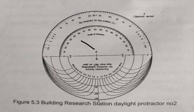
Each protractor consists of two scales: ‘A’ giving an initial reading (from sections of the room) and ‘B’ giving a correction factor (from plans).
The initial reading would give the sky component for infinitely long windows, but for a window of finite length (width) a correction factor (scale B) must be applied. Protractor 2 is illustrated in Figure 5.3.